Neural Network Adder Function
A Neural Network Adder Function is the dot product between a Neural Network Input vector and a Neural Network Weight matrix.
- AKA: Neuron Adder Function, Neuron Summing Function, Neuron Activation Potential, Neuron Net Input Function.
- Context:
- It can be defined as
[math]\displaystyle{ \varphi(X,W)=W^T\dot X \quad \Longleftrightarrow \quad \varphi_j=\sum_{i=1}^Px_iw_{ij} }[/math]
where [math]\displaystyle{ X \in \mathbb{R}^P }[/math] is neural network input vector, [math]\displaystyle{ W \in \mathbb{R}^{M \times P} }[/math] the neural network weight vector/matrix.
- It can also be defined as
[math]\displaystyle{ \varphi(X,W)=W^T\dot X + b \quad \Longleftrightarrow \quad \varphi_j=\sum_{i=1}^Px_iw_{ij}+b }[/math]
when a bias neuron is taken into consideration.
- It can be defined as
- Example(s):
- [math]\displaystyle{ \varphi=x_1w_1+x_2w_2+x_3w_2 +b }[/math] is a neuron adder function for a Neural Network Layer with 3 inputs and 1 output.
- [math]\displaystyle{ \begin{pmatrix} \varphi_1 \\ \varphi_2 \\ \vdots \\ \varphi_p \end{pmatrix} = \begin{pmatrix} w_{11} & w_{21} & \cdots & w_{p1} \\ w_{12} & w_{22} & \cdots & w_{p2} \\ \vdots & \vdots & \ddots & \vdots \\ w_{1n} & w_{2n} & \cdots & w_{pn} \end{pmatrix}*\begin{pmatrix} x_1 \\ x_2 \\ \vdots \\ x_n \end{pmatrix}+b }[/math] are neuron adder functions for a Neural Network Layer with n inputs and p outputs.
- …
- Counter-Example(s):
- See: Artificial Neural Network, Artificial Neuron, Neural Network Topology, Neural Network Layer.
References
2018
- (CS231n, 2018) ⇒ Biological motivation and connections. In: CS231n Convolutional Neural Networks for Visual Recognition Retrieved: 2018-01-14.
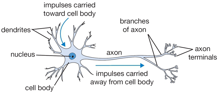
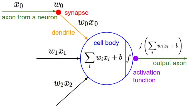
- QUOTE: The basic computational unit of the brain is a neuron. Approximately 86 billion neurons can be found in the human nervous system and they are connected with approximately [math]\displaystyle{ 10^{14} - 10^{15} }[/math] synapses. The diagram below shows a cartoon drawing of a biological neuron (left) and a common mathematical model (right). Each neuron receives input signals from its dendrites and produces output signals along its (single) axon. The axon eventually branches out and connects via synapses to dendrites of other neurons. In the computational model of a neuron, the signals that travel along the axons (e.g. [math]\displaystyle{ x_0 }[/math]) interact multiplicatively (e.g. [math]\displaystyle{ w_0x_0 }[/math]) with the dendrites of the other neuron based on the synaptic strength at that synapse (e.g. [math]\displaystyle{ w_0 }[/math]). The idea is that the synaptic strengths (the weights [math]\displaystyle{ w }[/math]) are learnable and control the strength of influence (and its direction: excitory (positive weight) or inhibitory (negative weight)) of one neuron on another. In the basic model, the dendrites carry the signal to the cell body where they all get summed. If the final sum is above a certain threshold, the neuron can fire, sending a spike along its axon. In the computational model, we assume that the precise timings of the spikes do not matter, and that only the frequency of the firing communicates information. Based on this rate code interpretation, we model the firing rate of the neuron with an activation function [math]\displaystyle{ f }[/math], which represents the frequency of the spikes along the axon. Historically, a common choice of activation function is the sigmoid function [math]\displaystyle{ \sigma }[/math], since it takes a real-valued input (the signal strength after the sum) and squashes it to range between 0 and 1. We will see details of these activation functions later in this section.

 A cartoon drawing of a biological neuron (left) and its mathematical model (right).
- QUOTE: The basic computational unit of the brain is a neuron. Approximately 86 billion neurons can be found in the human nervous system and they are connected with approximately [math]\displaystyle{ 10^{14} - 10^{15} }[/math] synapses. The diagram below shows a cartoon drawing of a biological neuron (left) and a common mathematical model (right). Each neuron receives input signals from its dendrites and produces output signals along its (single) axon. The axon eventually branches out and connects via synapses to dendrites of other neurons. In the computational model of a neuron, the signals that travel along the axons (e.g. [math]\displaystyle{ x_0 }[/math]) interact multiplicatively (e.g. [math]\displaystyle{ w_0x_0 }[/math]) with the dendrites of the other neuron based on the synaptic strength at that synapse (e.g. [math]\displaystyle{ w_0 }[/math]). The idea is that the synaptic strengths (the weights [math]\displaystyle{ w }[/math]) are learnable and control the strength of influence (and its direction: excitory (positive weight) or inhibitory (negative weight)) of one neuron on another. In the basic model, the dendrites carry the signal to the cell body where they all get summed. If the final sum is above a certain threshold, the neuron can fire, sending a spike along its axon. In the computational model, we assume that the precise timings of the spikes do not matter, and that only the frequency of the firing communicates information. Based on this rate code interpretation, we model the firing rate of the neuron with an activation function [math]\displaystyle{ f }[/math], which represents the frequency of the spikes along the axon. Historically, a common choice of activation function is the sigmoid function [math]\displaystyle{ \sigma }[/math], since it takes a real-valued input (the signal strength after the sum) and squashes it to range between 0 and 1. We will see details of these activation functions later in this section.
2016
- (Zhao, 2016) ⇒ Peng Zhao, February 13, 2016. R for Deep Learning (I): Build Fully Connected Neural Network from Scratch
- QUOTE: A neuron is a basic unit in the DNN which is biologically inspired model of the human neuron. A single neuron performs weight and input multiplication and addition (FMA), which is as same as the linear regression in data science, and then FMA’s result is passed to the activation function. The commonly used activation functions include sigmoid, ReLu, Tanh and Maxout. In this post, I will take the rectified linear unit (ReLU) as activation function, f(x) = max(0, x). For other types of activation function, you can refer here.

In R, we can implement neuron by various methods, such as
sum(xi*wi). But, more efficient representation is by matrix multiplication.R code:
neuron.ij <- max(0, input %*% weight + bias)
- QUOTE: A neuron is a basic unit in the DNN which is biologically inspired model of the human neuron. A single neuron performs weight and input multiplication and addition (FMA), which is as same as the linear regression in data science, and then FMA’s result is passed to the activation function. The commonly used activation functions include sigmoid, ReLu, Tanh and Maxout. In this post, I will take the rectified linear unit (ReLU) as activation function, f(x) = max(0, x). For other types of activation function, you can refer here.
2005
- (Golda, 2005) ⇒ Adam Gołda (2005). Introduction to neural networks. AGH-UST.
- QUOTE: The scheme of the neuron can be made on the basis of the biological cell. Such element consists of several inputs. The input signals are multiplied by the appropriate weights and then summed. The result is recalculated by an activation function.

In accordance with such model, the formula of the activation potential [math]\displaystyle{ \varphi }[/math] is as follows
[math]\displaystyle{ \varphi=\sum_{i=1}^Pu_iw_i }[/math]
Signal [math]\displaystyle{ \varphi }[/math] is processed by activation function, which can take different shapes.
- QUOTE: The scheme of the neuron can be made on the basis of the biological cell. Such element consists of several inputs. The input signals are multiplied by the appropriate weights and then summed. The result is recalculated by an activation function.