Residual Neural Network (ResNet) Architecture
A Residual Neural Network (ResNet) Architecture is an deep neural network architecture that is based on batch normalization and consists of residual units which have skip connections.
- Context:
- It can range from a Shallow Residual Neural Network to being a Deep Residual Neural Network.
- It can be used to solve the vanishing gradient problem.
- …
- Example(s):
- Counter-Example(s):
- See: Feature (Machine Learning), Artificial Neural Network, Pyramidal Cell, Cerebral Cortex, Rectifier (Neural Networks), Batch Normalization, Highway Network, Vanishing Gradient Problem.
References
2021
- (Wikipedia, 2021) ⇒ https://en.wikipedia.org/wiki/Residual_neural_network Retrieved:2021-1-24.
- A residual neural network (ResNet) is an artificial neural network (ANN) of a kind that builds on constructs known from pyramidal cells in the cerebral cortex. Residual neural networks do this by utilizing skip connections, or shortcuts to jump over some layers. Typical ResNet models are implemented with double- or triple- layer skips that contain nonlinearities (ReLU) and batch normalization in between. An additional weight matrix may be used to learn the skip weights; these models are known as HighwayNets. Models with several parallel skips are referred to as DenseNets. In the context of residual neural networks, a non-residual network may be described as a plain network.
One motivation for skipping over layers is to avoid the problem of vanishing gradients, by reusing activations from a previous layer until the adjacent layer learns its weights. During training, the weights adapt to mute the upstream layer, and amplify the previously-skipped layer. In the simplest case, only the weights for the adjacent layer's connection are adapted, with no explicit weights for the upstream layer. This works best when a single nonlinear layer is stepped over, or when the intermediate layers are all linear. If not, then an explicit weight matrix should be learned for the skipped connection (a HighwayNet should be used).
Skipping effectively simplifies the network, using fewer layers in the initial training stages. This speeds learning by reducing the impact of vanishing gradients, as there are fewer layers to propagate through. The network then gradually restores the skipped layers as it learns the feature space. Towards the end of training, when all layers are expanded, it stays closer to the manifoldand thus learns faster. A neural network without residual parts explores more of the feature space. This makes it more vulnerable to perturbations that cause it to leave the manifold, and necessitates extra training data to recover.
- A residual neural network (ResNet) is an artificial neural network (ANN) of a kind that builds on constructs known from pyramidal cells in the cerebral cortex. Residual neural networks do this by utilizing skip connections, or shortcuts to jump over some layers. Typical ResNet models are implemented with double- or triple- layer skips that contain nonlinearities (ReLU) and batch normalization in between. An additional weight matrix may be used to learn the skip weights; these models are known as HighwayNets. Models with several parallel skips are referred to as DenseNets. In the context of residual neural networks, a non-residual network may be described as a plain network.
2020
- (GeeksforGeeks, 2020) ⇒ https://www.geeksforgeeks.org/introduction-to-residual-networks/
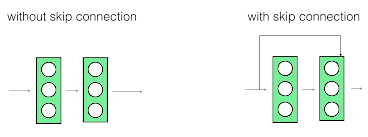
- QUOTE: The ResNet152 model with 152 layers won the ILSVRC Imagenet 2015 test while having lesser parameters than the VGG19 network, which was very popular at that time. A residual network consists of residual units or blocks which have skip connections, also called identity connections.
The skip connections are shown below:
- QUOTE: The ResNet152 model with 152 layers won the ILSVRC Imagenet 2015 test while having lesser parameters than the VGG19 network, which was very popular at that time. A residual network consists of residual units or blocks which have skip connections, also called identity connections.

|
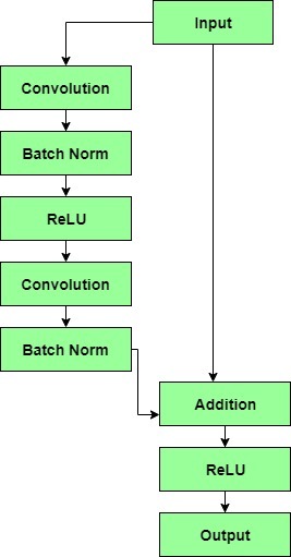
- The output of the previous layer is added to the output of the layer after it in the residual block. The hop or skip could be 1, 2 or even 3. When adding, the dimensions of $x$ may be different than $F(x)$ due to the convolution process, resulting in a reduction of its dimensions. Thus, we add an additional 1 × 1 convolution layer to change the dimensions of $x$.

|
- A residual block has a 3 × 3 convolution layer followed by a batch normalization layer and a ReLU activation function. This is again continued by a 3 × 3 convolution layer and a batch normalization layer. The skip connection basically skips both these layers and adds directly before the ReLU activation function. Such residual blocks are repeated to form a residual network.
2019
- (Alzantot et al., 2019) ⇒ Moustafa Alzantot, Ziqi Wang, and Mani B. Srivastava. (2019). “Deep Residual Neural Networks for Audio Spoofing Detection.” In: Proceedings of 20th Annual Conference of the International Speech Communication Association (Interspeech 2019).
- QUOTE: Figure 1 shows the architecture of the Spec-ResNet model which takes the log-magnitude STFT as input features. First, the input is treated as a single channel image and passed through a 2D convolution layer with 32 filters, where filter size = 3 × 3, stride length = 1 and padding = 1. The output volume of the first convolution layer has 32 channels and is passed through a sequence of 6 residual blocks. The output from the last residual block is fed into a dropout layer (with dropout rate = 50%; Srivastava et al., 2014) followed by a hidden fully connected (FC) layer with leaky-ReLU (He et al., 2015) activation function ($\alpha = 0.01$). Outputs from the hidden FC layer are fed into another FC layer with two units that produce classification logits. The logits are finally converted into a probability distribution using a final softmax layer.
- QUOTE: Figure 1 shows the architecture of the Spec-ResNet model which takes the log-magnitude STFT as input features. First, the input is treated as a single channel image and passed through a 2D convolution layer with 32 filters, where filter size = 3 × 3, stride length = 1 and padding = 1. The output volume of the first convolution layer has 32 channels and is passed through a sequence of 6 residual blocks. The output from the last residual block is fed into a dropout layer (with dropout rate = 50%; Srivastava et al., 2014) followed by a hidden fully connected (FC) layer with leaky-ReLU (He et al., 2015) activation function ($\alpha = 0.01$). Outputs from the hidden FC layer are fed into another FC layer with two units that produce classification logits. The logits are finally converted into a probability distribution using a final softmax layer.

|

|
2018
- (Li et al., 2018) ⇒ Juncheng Li, Faming Fang, Kangfu Mei, and Guixu Zhang. (2018). “Multi-scale Residual Network for Image Super-Resolution.” In: Proceedings of 15th European Conference in Computer Vision (ECCV 2018) - Part VIII.
- QUOTE: In order to detect the image features at different scales, we propose multi-scale residual block (MSRB). Here we will provide a detailed description of this structure. As shown in Fig. 3, our MSRB contains two parts: multi-scale features fusion and local residual learning.
- QUOTE: In order to detect the image features at different scales, we propose multi-scale residual block (MSRB). Here we will provide a detailed description of this structure. As shown in Fig. 3, our MSRB contains two parts: multi-scale features fusion and local residual learning.

|
2016a
- (He et al., 2016) ⇒ Kaiming He, Xiangyu Zhang, Shaoqing Ren, and Jian Sun. (2016). “Deep Residual Learning for Image Recognition.” In: Proceedings 2016 IEEE Conference on Computer Vision and Pattern Recognition (CVPR 2016).
- QUOTE: The formulation of $F(x) +x$ can be realized by feedforward neural networks with “shortcut connections” (Fig. 2). Shortcut connections (Bishop, 1995; Ripley, 1996, Venables & Ripley, 1999) are those skipping one or more layers. In our case, the shortcut connections simply perform identity mapping, and their outputs are added to the outputs of the stacked layers (Fig. 2). Identity shortcut connections add neither extra parameter nor computational complexity. The entire network can still be trained end-to-end by SGD with backpropagation, and can be easily implemented using common libraries (e.g., Caffe Jia et al., 2014) without modifying the solvers.
- QUOTE: The formulation of $F(x) +x$ can be realized by feedforward neural networks with “shortcut connections” (Fig. 2). Shortcut connections (Bishop, 1995; Ripley, 1996, Venables & Ripley, 1999) are those skipping one or more layers. In our case, the shortcut connections simply perform identity mapping, and their outputs are added to the outputs of the stacked layers (Fig. 2). Identity shortcut connections add neither extra parameter nor computational complexity. The entire network can still be trained end-to-end by SGD with backpropagation, and can be easily implemented using common libraries (e.g., Caffe Jia et al., 2014) without modifying the solvers.

|
2016b
- (He et al., 2016) ⇒ Kaiming He, Xiangyu Zhang, Shaoqing Ren, and Jian Sun. (2016). “Identity Mappings in Deep Residual Networks.” In: Proceedings of the 14th European Conference on Computer Vision (ECCV 2016) Part IV. DOI:10.1007/978-3-319-46493-0_38.
- QUOTE: Though our above analysis is driven by identity $f$, the experiments in this section are all based on $f = ReLU$ as in (He et al., 2016); we address identity $f$ in the next section. Our baseline ResNet-110 has 6.61% error on the test set. The comparisons of other variants (Fig. 2 and Table 1) are summarized as follows:
(...)
- QUOTE: Though our above analysis is driven by identity $f$, the experiments in this section are all based on $f = ReLU$ as in (He et al., 2016); we address identity $f$ in the next section. Our baseline ResNet-110 has 6.61% error on the test set. The comparisons of other variants (Fig. 2 and Table 1) are summarized as follows:

|

|

|
2016c
- (Zagoruyko & Komodakis, 2016) ⇒ Sergey Zagoruyko, and Nikos Komodakis. (2016). “Wide Residual Networks.” In: Proceedings of the British Machine Vision Conference 2016 (BMVC 2016).
- QUOTE: Residual block with identity mapping can be represented by the following formula:
| [math]\displaystyle{ \mathbf{x}_{l+1}=\mathbf{x}_{l}+\mathcal{F}\left(\mathbf{x}_{l}, \mathcal{W}_{l}\right) }[/math] | (1) |
- where $\mathbf{x}_{l+1}$ and $\mathbf{x}_{l}$ are input and output of the $l$-th unit in the network, $\mathcal{F}$ is a residual function and $\mathcal{W}_{l}$ are parameters of the block. Residual network consists of sequentially stacked residual block.
- where $\mathbf{x}_{l+1}$ and $\mathbf{x}_{l}$ are input and output of the $l$-th unit in the network, $\mathcal{F}$ is a residual function and $\mathcal{W}_{l}$ are parameters of the block. Residual network consists of sequentially stacked residual block.

|