Bidirectional LSTM (BiLSTM) Training Task
(Redirected from BiLSTM training task)
Jump to navigation
Jump to search
A Bidirectional LSTM (BiLSTM) Training Task is a Bidirectional Neural Network Training Task that contains LSTM units.
- AKA: BLSTM Training Task, BiLSTM Training Task.
- Example(s):
- Counter-Example(s):
- See: Bidirectional LSTM (biLSTM) Network, LSTM Training System, RNN Training System, Artificial Neural Network, PyTorch.
References
2018a
- (Cui, Ke & Wang, 2018) ⇒ Zhiyong Cui, Ruimin Ke, and Yinhai Wang (2018). "Deep Bidirectional and Unidirectional LSTM Recurrent Neural Network for Network-wide Traffic Speed Prediction" (PDF). arXiv preprint [arXiv:1801.02143].
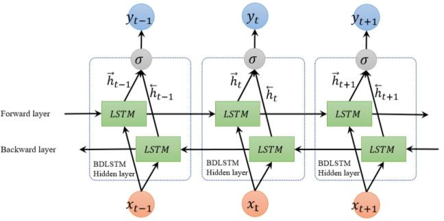
- QUOTE: ... the structure of an unfolded BDLSTM layer, containing a forward LSTM layer and a backward LSTM layer, is introduced and illustrated in Fig. 3.

Fig. 3 Unfolded architecture of bidirectional LSTM with three consecutive steps
2018b
- (Github, 2018) ⇒ Theano-Recurrence Training System: https://github.com/uyaseen/theano-recurrence training Retrieved: 2018-07-01
train.pyprovides a convenient methodtrain(..)to train each model, you can select the recurrent model with therec_modelparameter, it is set togruby default (possible options includernn,gru,lstm,birnn,bigru&bilstm), number of hidden neurons in each layer (at the moment only single layer models are supported to keep the things simple, although adding more layers is very trivial) can be adjusted byn_hparameter intrain(..), which by default is set to100. As the model is trained it stores the current best state of the model i.e set of weights (best = least training error), the stored model is in thedata\models\MODEL-NAME-best_model.pkl, also this stored model can later be used for resuming training from the last point or just for prediction/sampling. If you don't want to start training from scratch and instead use the already trained model then setuse_existing_model=Truein argument totrain(..). Also optimization strategies can be specified totrain(..)via optimizer parameter, currently supported optimizations arermsprop,adamandvanilla stochastic gradient descentand can be found inutilities\optimizers.py.b_path,learning_rate,n_epochsin thetrain(..)specifies the'base path to store model' (default = data\models\),'initial learning rateof the optimizer', and 'number of epochs respectively'. During the training some logs (current epoch, sample, cross-entropy error etc) are shown on console to get an idea of how well learning is proceeding, logging frequencycan be specified vialogging_freqin thetrain(..). At the end of training, a plot ofcross-entropy error vs # of iterationsgives an overview of overall training process and is also stored in theb_path.
2015
- (Fan et al., 2015) ⇒ Bo Fan, Lijuan Wang, Frank K. Soong, and Lei Xie (2015, April). "Photo-real talking head with deep bidirectional LSTM". In Acoustics, Speech and Signal Processing (ICASSP), 2015 IEEE International Conference on (pp. 4884-4888). IEEE. DOI: 10.1109/ICASSP.2015.7178899
- QUOTE: In our BLSTM network, as shown in Fig. 3, label sequence [math]\displaystyle{ L }[/math] is the input layer, and visual feature sequence [math]\displaystyle{ V }[/math] serves as the output layer and [math]\displaystyle{ H }[/math] denotes the hidden layer. In particular, at t-th frame, the input of the network is the t-th label vector [math]\displaystyle{ l_t }[/math] and the output is the [math]\displaystyle{ t }[/math]-th visual feature vector [math]\displaystyle{ v_t }[/math]. As described in (Graves, 2012), the basic idea of this bidirectional structure is to present each sequence forwards and backwards to two separate recurrent hidden layers, both of which are connected to the same output layer. This provides the network with complete, symmetrical, past and future context for every point in the input sequence. Please note that in Fig. 3, more hidden layers can be added in to construct a deep BLSTM.
In the training stage, we have multiple sequence pairs of [math]\displaystyle{ L }[/math] and [math]\displaystyle{ V }[/math]. As we represent both sequences as continuous numerical vectors, the network is treated as a regression model to minimizing the SSE of predicting [math]\displaystyle{ \hat{V} }[/math] from [math]\displaystyle{ L }[/math].

Fig. 3. BLSTM neural network in our talking head system.
- QUOTE: In our BLSTM network, as shown in Fig. 3, label sequence [math]\displaystyle{ L }[/math] is the input layer, and visual feature sequence [math]\displaystyle{ V }[/math] serves as the output layer and [math]\displaystyle{ H }[/math] denotes the hidden layer. In particular, at t-th frame, the input of the network is the t-th label vector [math]\displaystyle{ l_t }[/math] and the output is the [math]\displaystyle{ t }[/math]-th visual feature vector [math]\displaystyle{ v_t }[/math]. As described in (Graves, 2012), the basic idea of this bidirectional structure is to present each sequence forwards and backwards to two separate recurrent hidden layers, both of which are connected to the same output layer. This provides the network with complete, symmetrical, past and future context for every point in the input sequence. Please note that in Fig. 3, more hidden layers can be added in to construct a deep BLSTM.