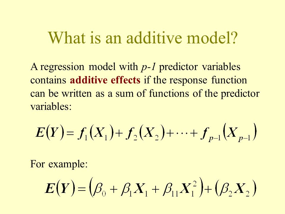
Additive Model (AM) Function

An Additive Model (AM) Function is a model function of the form [math]\displaystyle{ Y= \beta_0+\sum_{j=1}^p f_j(X_{j})+\varepsilon }[/math].

Context:
- It can be trained by an Additive Model Training System.
- It can (typically) be an Interpretable Model.
- …
See: Additive Tree, Additive Modeling, Interaction Regression Model, Statistical Unit, Smooth Function, Backfitting Algorithm.

References

(Wikipedia, 2020) ⇒ https://en.wikipedia.org/wiki/Additive_model Retrieved:2020-10-2.
- In statistics, an additive model (AM) is a nonparametric regression method. It was suggested by Jerome H. Friedman and Werner Stuetzle (1981) ^[1] and is an essential part of the ACE algorithm. The AM uses a one-dimensional smoother to build a restricted class of nonparametric regression models. Because of this, it is less affected by the curse of dimensionality than e.g. a p-dimensional smoother. Furthermore, the AM is more flexible than a standard linear model, while being more interpretable than a general regression surface at the cost of approximation errors. Problems with AM include model selection, overfitting, and multicollinearity.

(Wikipedia, 2020) ⇒ https://en.wikipedia.org/wiki/Additive_model#Description Retrieved:2020-10-2.
- Given a data set [math]\displaystyle{ \{y_i,\, x_{i1}, \ldots, x_{ip}\}_{i=1}^n }[/math] of n statistical units, where [math]\displaystyle{ \{x_{i1}, \ldots, x_{ip}\}_{i=1}^n }[/math] represent predictors and [math]\displaystyle{ y_i }[/math] is the outcome, the additive model takes the form :
  [math]\displaystyle{ E[y_i|x_{i1}, \ldots, x_{ip}] = \beta_0+\sum_{j=1}^p f_j(x_{ij}) }[/math]
  or
  [math]\displaystyle{ Y= \beta_0+\sum_{j=1}^p f_j(X_{j})+\varepsilon }[/math] Where [math]\displaystyle{ \lt P\gt E[ \epsilon ] = 0 }[/math] , [math]\displaystyle{ Var(\epsilon) = \sigma^2 }[/math] and [math]\displaystyle{ E[ f_j(X_{j}) ] = 0 }[/math] . The functions [math]\displaystyle{ f_j(x_{ij}) }[/math] are unknown smooth functions fit from the data. Fitting the AM (i.e. the functions [math]\displaystyle{ f_j(x_{ij}) }[/math] ) can be done using the backfitting algorithm proposed by Andreas Buja, Trevor Hastie and Robert Tibshirani (1989). ^[2]

↑ Friedman, J.H. and Stuetzle, W. (1981). "Projection Pursuit Regression", Journal of the American Statistical Association 76:817–823.
↑ Buja, A., Hastie, T., and Tibshirani, R. (1989). "Linear Smoothers and Additive Models", The Annals of Statistics 17(2):453–555.